
Kalman filtering of IMU data
Introduction
To many of us, kalman filtering is something like the holy grail. Indeed, it miraculously solves some problems which are otherwise hard to get a hold on. But beware, kalman filtering is not a silver bullet and won’t solve all of your problems!
This article will explain how Kalman filtering works. We’ll use a more practical approach to avoid the boring theory, which is hard to understand anyway. Since most of you will only use it for MAV/UAV applications, I’ll try to make it look more concrete instead of puzzling generalized approach.
Make sure you know from the previous articles how the data from “accelerometers” and “gyroscopes” are used. Some basic knowledge of algebra may also come in handy :-)
Basic operation
Kalman filtering is an iterative filter that requires two things.
First of all, you will need some kind of input (from one or more sources) that you can turn into a prediction of the desired output using only linear calculations. In other words, we will need a lineair model of our problem.
Secondly, you will need another input. This can be the real world value of the predicted one, or something that is a good approximation of it.
Every iteration, the kalman filter will change the variables in our lineair model a bit, so the output of our linear model will be closer to the second input.
Our simple model
Obviously, our two inputs will consist of the gyroscope and accelerometer data. The model using the gyroscope data looks like this:
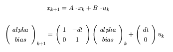
The first formula represents the general form of a linear model. We need to “fill in” the A en B matrix, and choose a state x. The variable u represents the input. In our case this will be the gyroscope’s data. Remember how we integrate? We just add the NORMALIZED measurements up:
alpha k = alpha k-1 + (_u_ k – bias)
We need to include the time between two measurements (_dt_) because we are dealing with the rate (degrees/s):
alpha k = alpha k-1 + (_u_ k – bias) * dt
We rewrite it:
alpha k = alpha k-1 – bias * dt + u k * dt
Which is what we have in our matrix multiplication. Remark that our bias remains constant! In the tutorial on gyroscopes, we saw that the bias drifts. Well, here comes the kalman-magic: the filter will adjust the bias in each iteration by comparing the result with the accelerometer’s output (our second input)! Great!
Wrapping it all up
Now all we need are the bits and bolts that actually do the magic! These are some formulas using matrix algebra and statistics. No need right now to know the details of it. Here they are:
| u = measurement1 | Read the value of the last measurement |
| x = A · x + B · u | Update the state x of our model |
| y = measurement2 | Read the value of the second measurement/real value. Here this will be the angle calculated from our accelerometer. |
| Inn = y – C · x | Calculate the difference between the second value and the value predicted by our model. This is called the innovation |
| s = C · P · C’ + Sz | Calculate the covariance |
| K = A · P · C’ · inv(_s_) | Calculate the kalman gain |
| x = x + K · Inn | Correct the prediction of the state |
| P = A · P · A’ – K · C · P · A’ + Sw | Calculate the covariance of the prediction error |
The C matrix is the one that extracts the ouput from the state matrix. In our case, this is (1 0)’ :
alpha = C · x
Sz is the measurement process noise covariance: Sz = E(zk zkT)
In our example, this is how much jitter we expect on our accelerometer’s data.
Sw is the process noise covariance matrix (a 2×2 matrix here): Sw = E(x · xT)
Thus: Sw = E( [alpha bias]’ · [alpha bias] )
Since only the diagonal elements of the Sw matrix are being used, we’ll only need to know E(alpha2) and E(bias2), which is the 2nd moment. To calculate those values, we’ll need to look at our model: The noise in alpha comes from the gyroscope and is multiplied by dt2. Thus: E(alpha2) = E(u2)· dt2.
These factors depend on the sensors you’re using. You’ll need to figure them out by doing some experiments. In the source code of the autopilot/rotomotion kalman filtering, they use the following constants:
E(alpha2) = 0.001
E(bias2) = 0.003
Sz = 0.3 (radians = 17.2 degrees)
Further reading
|