MAV-blog

Now you know most practical things you need to know about accelerometers, we’ll continue with gyroscopes (other names: gyro, angular rate sensor).

A gyroscope is a very fancy name for a device that measures the angular rate (how much degrees per second it is rotating). The gyroscopes used in very critical applications (like a jumbo jet) are very advanced and complicated. Fortunately for us, there are some low-cost and small sized alternatives which are good enough. They are fabricated using MEMS (iMEMS) technology by big companies like Analog Devices.
Great! Let’s start with some theory:

As you probably remember from you physics class, position, velocity and acceleration are related to eachother: deriving the position, gives us velocity:

d x = v _x

with x being the position on the x-axis and v _x being the velocity along the x-axis.
Maybe less obvious, the same holds for angles. While velocity is the speed at which the position is changing, angular rate is nothing more than the speed the angle is changing. That’s right:

d alpha = angular rate = gyroscope output

with alpha being the angle. It’s starting to look pretty good! Knowing that the inverse of deriving (d .) is integrating (∫), we change our formula’s into:

∫ angular rate = ∫ gyroscope output = alpha

Woohoo, we found a relation between angle (attitude!) and our gyroscope’s output: integrating the gyroscope, gives us our attitude-angle.

Enough boring theory! Let’s take a look at some figures. The following figures all represent the same motion: I took a gyroscope, turned it 90 degrees left and back, and turned it 90 degrees right and back.

The raw data (used here) is what we get when we feed the gyroscope’s output (0-5 volt) into a 10-bit ADC (analog to digital convertor). So the raw values are between 0 and 1024. Here’s a figure of that:

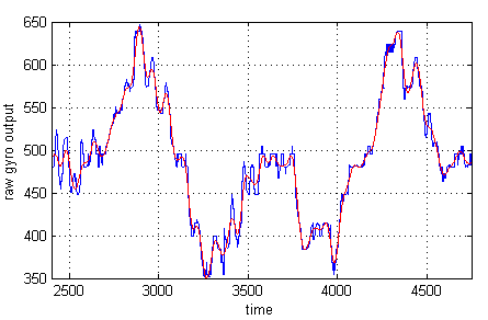
(The red line is just a low-pass filtered version of the blue data)
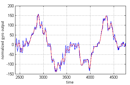
You can clearly see a positive angular rate followed by a negative one. But we’ll need to shift the figure down, to make sure negative values correspond to a negative angular rate. Otherwise the integration (which can be seen as the sum of our y-values) would keep adding up values and never substracting any! We normalize it by substracting about 490 from every value. This normalization gives us the following figure:

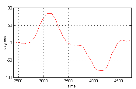
Now all we need to do, according to our formulas, is integrate it! Some of you may still have nightmares about college and start shivering when they hear the word integration, but its pretty simple. Discrete integration is nothing more than summing up all the values! Basically, integration from 0 to the i^th^ value:

integration(i) = integration (i-1) + val_i

This is the simplest possible integrator. A more advanced one, which also flattens out possible jitter in the data, is the runge-kutta integrator:

integration(i) = integration(i-1) + ¹⁄₆ ( val_i-3 + 2 val_i-2 + 2 val_i-1 + val_i)

Using this runge-kutta integration, we get the following figure:

This is pretty much the exact movement I made! Now we just need to add a scale factor to our data so our result is in degrees:

This pretty much ends my story of the simplified gyroscope!

In reality, gyroscopes are suffering from an effect called drift. This means that over time, the value a gyroscope has when in steady position (called bias), drifts away from it’s initial steady value:

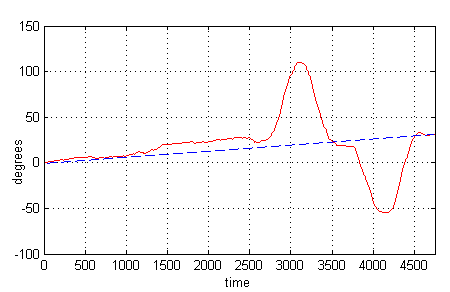
The blue line gives you an idea about the drift. During 4500 samples (12 seconds in my setup), the bias drifted about 30 degrees!

Remember that we need the bias (about 490 in our example) to normalize our data. How can we integrate when we have no idea about the currect bias? We’ll need to find a way to get it. More about this in the next article. A hint: our accelerometer isn’t affected by drift ;-)